


Theoretical Background & Model Development in DSHplus
The different types of cavitation are represented by suitable mathematical models within the simulation framework DSHplus.
On this page, you'll find out how...
- Vapour cavitation
- Pressure-dependent gas absorption capability
- Gas absorption & resorption rates
- Gas transport
- Impact of finite gas fractions on fluid properties
- Choking in resistors
- Gas desorption in resistors
...is modelled in DSHplus.
The content of this page can be viewed in Webinar form by clicking on the adjacent video.
Vapour Cavitation
The calculation of vapour cavitation within the pipes is based on the “Discrete Vapour Cavity Model” (DVCM). This approach is probably the most commonly used model for 1D calculation of flows with vapour cavitation.
Fundamental assumptions:
- Instantaneous conversion of liquid to vapour once vapour pressure is reached
- Spatial dimensions of vapour bubbles are negligible for the analysis
- Vapour bubbles are not transported
- Cavitation is modelled as an isothermal process since the mass of the vapourised phase is very small
Procedure:
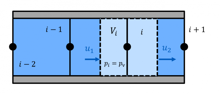
- Calculate pressures & velocities at node i as "usual", i.e. for cavitation-free flow.
- If the pressure at the node drops below vapour pressure, it is set to vapour pressure.
- Based on the prescribed vapour pressure at the node, the fluid velocities u1 and u2 are calculated.
- The difference between these two velocities is proportional to the temporal change of vapour volume Vv.
- The volumetric vapor fraction αv is then given by the ratio of vapour volume Vv and control volume Vi.
Advantage of the DVCM: The only required input parameter is the temperature-dependent vapour pressure of the liquid!
Pressure-dependent Gas Absorption Capability
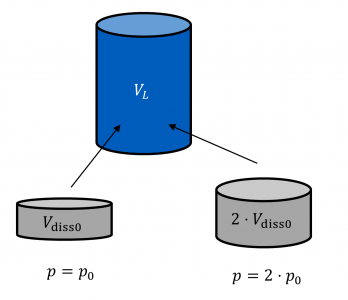
The capability of a liquid to dissolve a gas is characterised through the Bunsen coefficient αB.
The Bunsen coefficient indicates how much gas volume Vdiss0 can be absorbed by a liquid volume VL at ambient pressure p0.
The capability to dissolve gases is pressure-dependent (Henry's law). For pressures p ≠ p0, the gas volume that can be dissolved is given by:
$$V_\mathrm{diss0} = \frac{p}{p_0}\alpha_\mathrm{B}V_\mathrm{L}$$
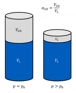
Hence, for a piston filled with hydraulic fluid and undissolved gas at ambient pressure, the volume VG of undissolved gas will decrease with increasing pressure, even if the gas were incompressible (see adjacent figure)!
If the fraction of undissolved gas at ambient pressure is referred to as αG0, the fraction αG(p) of undissolved gas at any pressure p is given by (note that αG still refers to ambient conditions!):
$$\alpha_\mathrm{G}(p) = \alpha_\mathrm{G0}+\alpha_\mathrm{B}\left(1-\frac{p}{p_0}\right)$$
If the mixture is compressed further, the gas fraction will be entirely dissolved above the pressure pα mentioned earlier:
$$p_\alpha = p_0 \left(1+\frac{\alpha_\mathrm{G0}}{\alpha_\mathrm{B}}\right)$$
However, the outlined behavior can only be observed for quasi-static (very slow) changes of the pressure.
Gas Absorption & Desorption Rates
In case of rapid pressure changes, the finite absorption and desorption rates of the gas fractions must be taken into account!
The temporal absorption or desorption behaviour of the liquid-gas mixture is modelled as a 1st order lag element (PT1) at the internal grid points of the pipe.
The parameters of the absorption and desorption functions (time constants τAbs and τDes) are system specific and must be determined experimentally; the standard parameters of DSHplus provide a rough orientation if no values are known.
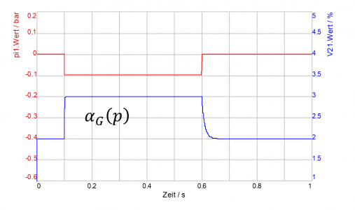
The effects of the time-dependent absorption or desorption are shown for exemplary selected parameters (τAbs =10 ms, τDes =1 ms) in the adjacent DSHplus screenshot.
It can be seen that (according to the parameterisation) the proportion of undissolved gas increases rapidly (desorption) when the pressure is lowered, but that the absorption of the gas back into the liquid occurs with a certain delay when the pressure rises again.
Gas Transport
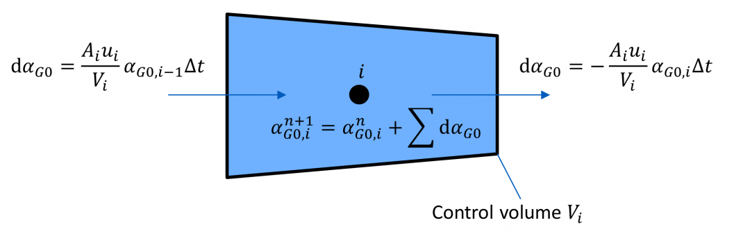
A homogenous mixture is assumed, thus dissolved and undissolved gas are transported with fluid velocity.
A control volume Vi corresponds to each grid point of the method of characteristics (MOC) grid.
The gas mass fraction (or the equivalent fraction of undissolved gas αG0 at reference pressure p0) at the new time step n + 1 is calculated from the incoming and outgoing mixture fluxes with their corresponding gas mass fractions.
Impact of Finite Gas Fractions on Fluid Properties
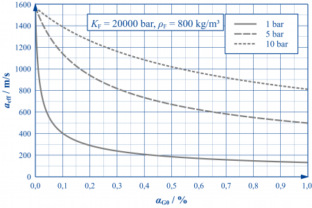
Where gas bubbles occur, the properties of the hydraulic fluid (more precisely: the fluid-gas mixture) undergo significant changes. Since the gas phase can be compressed much more easily than the liquid phase, the stiffness of the mixture - characterised by the effective bulk modulus Keff or the effective speed of sound aeff - is significantly lower than that of the "pure" liquid.
As the adjacent figure shows, even the smallest volume fractions of undissolved air are capable of drastically reducing the speed of sound in hydraulic oils. As the pressure level increases, the influence of undissolved air decreases as the bubble stiffness increases in proportion to the pressure.
The curves shown are only valid for slow processes. For highly dynamic processes (e.g. pressure surges), the frequency dependence of the gas bubble stiffness must also be taken into account. This can – depending on the frequency position – further reduce or even increase the stiffness of the mixture.
Choking in Resistors
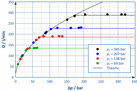
In general, the flow rate across a resistor increases with increasing pressure difference. However, this only applies as long as the flow is cavitation-free. If the pressure drops below the vapour pressure, vapour bubbles occur. The more vapour is generated, the more the flow through the resistor is constricted. A "saturation" of the flow rate can be observed – a larger pressure difference no longer leads to an increase in flow rate.
One could assume that the pressure difference across the resistance is the only parameter that determines the beginning and extent of cavitation. However, since – as shown in the adjacent figure – the occurrence of cavitation can be delayed by increasing the inlet pressure, this variable cannot be the only relevant parameter [1].
In practice, the combined effects of these two "set screws" are therefore determined by the cavitation index C (or its reciprocal value) [1]:
$$C=\frac{p_1-p_\mathrm{v}}{p_1-p_2}$$
Smaller values of the cavitation index C make the occurrence of cavitation more probable. Cavitation occurs when the cavitation index falls below a component-specific critical value Ckrit.
The measured values published by EBRAHIMI et al. can be reproduced in the 1D simulation with high accuracy by using a valve-specific typical value for Ckrit (dashed curves in the adjacent figure).
Gas Release in Resistors
If cavitation occurs at a resistor and the liquid carries dissolved gas, a certain amount of the gas is released due to gas cavitation.
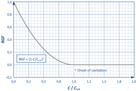
The amount of gas released by cavitation is described through the released gas fraction RGF, which is defined as follows:
$$RGF=\frac{\mathrm{Released\,volume\,fraction\,of\,gas}}{\mathrm{Incoming\,dissolved\,volume\,fraction\,of\,gas}}$$
If all the gas is released in the resistance, RGF takes on a value of one.
Since the relationship between the geometry of the resistor, the pressure drop and the amount of gas released is generally complex and situation-specific, the corresponding values must be determined either by experiment or through numerical 2D/3D simulation.
In order to enable a rough parameterisation – if no data is available – a pre-parameterised, semi-empirical model is available in DSHplus (see adjacent figure).
Literature
[1] EBRAHIMI, B. et al. „Characterization of high-pressure cavitating flow through a thick orifice plate in a pipe of constant cross section.“ International Journal of Thermal Sciences 114 (2017): 229-240.